Last post we got an idea of how Newton-Raphson works (and how similar it is to the one dimensional version). Here we will explore step by step how the algorithm works and how quickly it arrives to our minimum. We will be using the same function as before so we can compare how quickly the method descends. Here is our function in both a surface plot and a contour plot as a reminder. (f(x,y) = x^2 -x+cos(y+x)+y^2
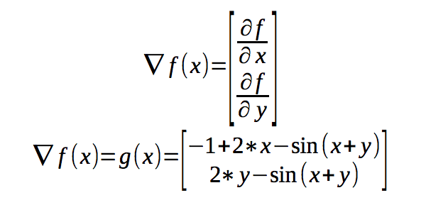
As you can see it is a relatively simple surface and convex. In order to use Newton Raphson, we need to take both the gradient and the hessian of our function. A quick mathematics reminder, The gradient is the vector which contains first derivatives of the function with respect to each of its variables. Below you can see a general case for the gradient as well our specific gradient for this function.
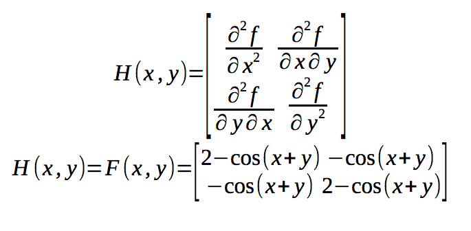
As I mentioned last post we also need the equivalent of the second derivative for newton-raphson. This takes the form of the hessian. Another quick mathematics reminder, the Hessian is the square matrix consisting of all the second derivatives of our function. The Hessian exhaustively takes the derivatives of the function with respect to one variable an d the second derivative with respect to every variable again. To clarify this i have left the general case below along with our specific case.
Note that the Hessian above is a square matrix (it always should be). The second check that has to be made is to ensure that the Hessian is invertible. Since we are dealing with matrix we cannot “divide” matrices, we must use the inverse of the Hessian instead. This comes into play with our iterative step. Now to start our method we need an initial point, we are going to use the same one as we did with Steepest Descent (8,8). With these values we calculate our Hessian and Gradient which gives us the following.  We now take the inverse of the Hessian and then find our next point. The iterative equation is listed below as well as the output.
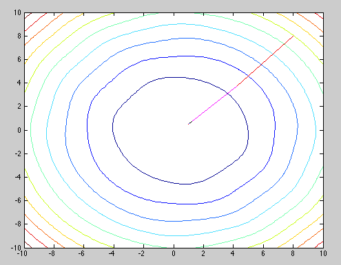
Our new point was a considerable decrease from our starting point. We repeat the above steps until we reach our stopping conditions which I set as our normal tolerance limits. I allowed the method to iterate until these conditions were met. The steps are outlined in the plot below.
The graph above looks similar to our dynamic steepest descent. As you can see the method was very direct. Taking only 5 iterations our method produces a minimum of (0.9987,0.4987). This is pretty much dead on to the actual minimum of our function. Newton Raphson makes quick work of the minimization. Next post we will look at the limitations of this method. Code below.
-Marcello
%newton raphson in  dimensions
%f(x,y) =  x^2 -x+cos(y+x)+y^2

x=zeros(2,7);
z=zeros(1,7);

x(1,1)=8; %initial guess
x(2,1)=8;


tol(1)=1;
tol(2)=2;

i=2;


while tol(1) >0.0001 && tol(2) > 0.0001 %stop conditions

    %gradients
    dx1 = -1+2*x(1,i-1)-sin(x(1,i-1)+x(2,i-1)); %gradient dx
    dx2 = 2*x(2,i-1) - sin(x(1,i-1)+x(2,i-1)); %gradient dy

    g=[dx1,dx2]';%gradient matrix

    %hessian
    ddx1= 2 - cos(x(1,i-1)+x(2,i-1)); % sames as ddx2
    dx1dx2= -cos(x(1,i-1)+x(2,i-1)); % same as dx2dx1

    h =[ddx1 dx1dx2;dx1dx2,ddx1]; %hessian matrix

    x(:,i) = x(:,i-1)-h\g;


    tol(1) = abs(x(1,i)-x(1,i-1)); %tolerance calc
    tol(2) = abs(x(2,i)-x(2,i-1));

    z(i) =x(1,i)^2 -x(1,i)+cos(x(2,i)+x(1,i))+x(2,i)^2; % function eval

    i=i+1;
end


